Sharing notes from my ongoing learning journey — what I build, break and understand along the way.
Understanding the Cost Function in Linear Regression with Real Examples
Linear Regression and the Cost Function: Step-by-Step Guide with Calculations
As someone who is just beginning to explore the field of artificial intelligence, I’ve realized that it’s not enough to focus solely on large models — I also need to understand the foundational building blocks behind them. That’s why I’m documenting my learning process step by step, creating content that serves both as a personal reference and a resource for others on a similar path.
In this post, we’ll explore one of the core components of linear regression: the cost function, using a hands-on, example-based approach with detailed calculations.
Linear Regression with One Variable – What Is the Cost Function?
Let’s say you’re given a list:
- Each house has a square meter (m²) value
- And each house has a known price
Now you want to do something like this:
“If I know the square meter, can I write an equation that can roughly estimate the price?”
That equation is what we call linear regression — in other words, you’re trying to draw a straight line that fits the data.
But here’s the problem:
This line can’t perfectly pass through every data point.
The actual prices and your estimated prices won’t match exactly.
So naturally, the following question arises:
“How wrong are my predictions? How far off am I?”
The thing that measures this difference is called the cost function.
Why Do We Need a Cost Function?
Because you need a concrete way to measure how good (or bad) your model’s predictions are.
- If your predictions are very close to the actual values → Low cost
- If your predictions are far off → High cost
Goal: Minimize this cost.
What Does the Cost Function Do?
It checks each prediction (e.g., for 100 houses) one by one.
For every house:
- It calculates the difference between the predicted price and the actual price
- It takes the square of this difference (so negative and positive errors don’t cancel each other)
- Then it finds the average of all these squared differences
And finally, it says:
“Your average error is this much.”
That value is called the cost.
What is Linear Regression?
Linear regression models the relationship between variables using a straight line.
$$
\hat{y} = \theta_1 x + \theta_0
$$
And describe terms like this:
\( \hat{y} \) — predicted value
\( x \) — input (e.g., house size)
\( \theta_1 \) — slope (weight)
\( \theta_0 \) — intercept (bias)
What Is the Cost Function?
The cost function measures how accurate predictions are. The most common is Mean Squared Error (MSE):
$$
\text{MSE} = \frac{1}{n} \sum_{i=1}^{n}(y_i – \hat{y}_i)^2
$$
Training form (used in gradient descent):
$$
J(\theta) = \frac{1}{2n} \sum_{i=1}^{n}(y_i – \hat{y}_i)^2
$$
Example Dataset: 10 Houses
| House | Size (m²) | Price ($1000) |
|---|---|---|
| x1 | 80 | 200 |
| x2 | 90 | 220 |
| x3 | 100 | 240 |
| x4 | 110 | 265 |
| x5 | 120 | 280 |
| x6 | 130 | 300 |
| x7 | 140 | 320 |
| x8 | 150 | 340 |
| x9 | 160 | 360 |
| x10 | 170 | 385 |
Initial Model y=1.9x−5
Error Calculations
| House | x | Prediction $$y^\hat{y}y^$$ | Actual y | Error | Error² |
|---|---|---|---|---|---|
| x1 | 80 | 147.0 | 200 | -53.0 | 2809.0 |
| x2 | 90 | 166.0 | 220 | -54.0 | 2916.0 |
| x3 | 100 | 185.0 | 240 | -55.0 | 3025.0 |
| x4 | 110 | 204.0 | 265 | -61.0 | 3721.0 |
| x5 | 120 | 223.0 | 280 | -57.0 | 3249.0 |
| x6 | 130 | 242.0 | 300 | -58.0 | 3364.0 |
| x7 | 140 | 261.0 | 320 | -59.0 | 3481.0 |
| x8 | 150 | 280.0 | 340 | -60.0 | 3600.0 |
| x9 | 160 | 299.0 | 360 | -61.0 | 3721.0 |
| x10 | 170 | 318.0 | 385 | -67.0 | 4489.0 |
Prediction function:y = 1.9x - 5
Then:
$$
2809 + 2916 + 3025 + 3721 + 3249 + 3364 + 3481 + 3600 + 3721 + 4489 = 34375
$$
MSE: $$
\frac{34375}{10} = 3437.5
$$
Cost function: $$
J(\theta) = \frac{1}{2} \times 3437.5 = 1718.75
$$
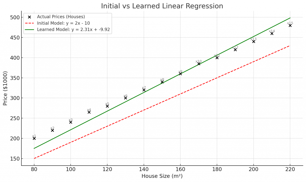
Learned Model y=2.31x−9.92
Error Calculations
| House | x | Prediction $$y^\hat{y}y^$$ | Actual y | Error | Error² |
|---|---|---|---|---|---|
| x1 | 80 | 174.88 | 200 | -25.12 | 630.98 |
| x2 | 90 | 198.98 | 220 | -21.02 | 442.02 |
| x3 | 100 | 223.08 | 240 | -16.92 | 286.20 |
| x4 | 110 | 247.18 | 265 | -17.82 | 317.53 |
| x5 | 120 | 271.28 | 280 | -8.72 | 76.03 |
| x6 | 130 | 295.38 | 300 | -4.62 | 21.34 |
| x7 | 140 | 319.48 | 320 | -0.52 | 0.27 |
| x8 | 150 | 343.58 | 340 | 3.58 | 12.81 |
| x9 | 160 | 367.68 | 360 | 7.68 | 59.01 |
| x10 | 170 | 391.78 | 385 | 6.78 | 45.97 |
Prediction function:y = 2.31x - 9.92
$$
630.98 + 442.02 + 286.20 + 317.53 + 76.03 + 21.34 + 0.27 + 12.81 + 59.01 + 45.97 = 2220.91
$$
MSE: $$
\frac{2220.91}{10} = 222.09
$$
Cost function: $$
J(\theta) = \frac{1}{2} \times 222.09 = 111.05
$$
The learned model reduces cost by more than 15x.
Graph Summary
- Black dots: actual prices
- Red dashed line: initial model
- Green line: learned model